Graphs
Shortest Path Algorithms
Pre-Requisite: Depth-First Search, Breadth-First Search
Finding shortest paths is one of the most fundamental graph problems. The algorithm you choose depends on one thing: what are the edge weights?
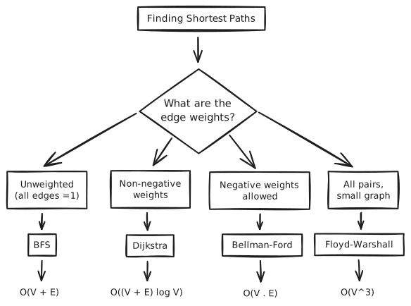
Let's have a look on each algorithm below.
1. BFS: When All Edges Are Equal
If every edge has the same cost (or weight = 1), BFS is your shortest path algorithm. If you're unfamiliar with BFS, start with our BFS introduction.
How BFS Finds Shortest Paths
BFS explores nodes level by level using a queue. The first time you reach a node, you've found the shortest path to it and no other path can be shorter because all edges cost the same.
Why does this work? The queue processes nodes in order of discovery. Nodes discovered first (closer to source) get processed before nodes discovered later (farther from source). This layer-by-layer exploration guarantees shortest paths.
Walkthrough
Let's trace through BFS on this graph in the visual below, starting from node 0:
- Initialize: Set dist[0] = 0 and add 0 to the queue
- Process 0: Discover neighbors 1 and 2 → set dist[1] = 1, dist[2] = 1, add both to queue
- Process 1: Discover neighbor 3 → set dist[3] = 2
- Process 2: Neighbors 3 and 4 → 3 already visited, set dist[4] = 2
- Continue until queue empty
Notice how BFS finds all nodes at distance 1 before any node at distance 2. This layer-by-layer exploration is what guarantees shortest paths.
Initialize: set dist[0] = 0, enqueue 0
0 / 12
Click Show Code in the visualization above to see the whole implementation.
You might wonder: shouldn't we use min(dist[neighbor], dist[node] + 1) instead of just assigning? No -- the if neighbor not in distances check handles this. We only set a distance the first time we reach a node, and in BFS, the first discovery is always the shortest path (because we process all nodes at distance d before any node at distance d+1). Once a node has a distance, we skip it entirely. No relaxation needed.
Complexity
Time: O(V + E) as each node is dequeued once, and each edge is examined once when we check neighbors.
Space: O(V) as the queue can hold at most V nodes, and we store distances for V nodes.
When to Use BFS
- Grid navigation (moving up/down/left/right)
- Unweighted graph traversal
- Finding minimum number of steps/moves
Problems That Use BFS for Shortest Path
- Minimum Knight Moves is a classic grid BFS
- Rotting Oranges is a multi-source BFS
- 01-Matrix finds distance from each cell to nearest 0
If a problem asks for "minimum moves" or "shortest path" in a grid or unweighted graph, try BFS first. It's simpler and often sufficient.
2. Dijkstra's Algorithm: Non-Negative Weights
Dijkstra's is the most important shortest path algorithm for interviews. It handles graphs where edges have non-negative weights.
The idea is to always explore the cheapest unexplored node. We can use a min-heap (priority queue) to efficiently find it.
How Dijkstra Works
The key insight is relaxation: for each edge, we ask "can we reach this neighbor faster by going through the current node?" If yes, we update the distance and add the neighbor to the heap.
Walkthrough
Let's trace Dijkstra on this weighted graph below, starting from node 0. The edges are: 0→1 (weight 4), 0→2 (weight 1), 2→1 (weight 2), 2→3 (weight 5), 1→3 (weight 1), 3→4 (weight 3).
- Initialize: dist[0] = 0, all others = ∞. Heap = [(0, 0)]
- Pop (0, 0): Process node 0. Check edges:
- 0→1: dist[1] = 0 + 4 = 4. Add (4, 1) to heap.
- 0→2: dist[2] = 0 + 1 = 1. Add (1, 2) to heap.
- Pop (1, 2): Process node 2 (smallest distance!). Check edges:
- 2→1: 1 + 2 = 3 < 4. Update dist[1] = 3. Add (3, 1) to heap.
- 2→3: dist[3] = 1 + 5 = 6. Add (6, 3) to heap.
- Pop (3, 1): Process node 1. Check edges:
- 1→3: 3 + 1 = 4 < 6. Update dist[3] = 4. Add (4, 3) to heap.
- Pop (4, 3): Process node 3. dist[4] = 4 + 3 = 7. Add (7, 4) to heap.
- Continue until heap empty.
Notice how we found a shorter path to node 1: the direct path 0→1 costs 4, but going 0→2→1 costs only 3. Dijkstra discovered this by always processing the cheapest node first.
Initialize: set dist[0] = 0, push (0, 0) to min-heap
0 / 18
Why It Works
Dijkstra is greedy: it always processes the node with the smallest known distance. Because all edge weights are non-negative, once we've processed a node, we've found its shortest path. No later discovery can improve it as for any other path would have to go through a node with equal or greater distance, then add more non-negative weight.
Dijkstra fails with negative edge weights. If an edge can reduce the total cost, the greedy assumption breaks down and we might find a shorter path after we've already "finalized" a node.
Complexity
Time: O((V + E) log V) with a binary heap
- Each edge might trigger a heap push: O(E log V)
- Each pop from the heap is O(log V), with at most O(E) entries
Space: O(V + E) — O(V) for the distances map, and the heap can grow to O(E) since stale entries aren't removed
When to Use Dijkstra
- Weighted graphs with non-negative edges
- Finding shortest path from one source to all nodes
- Problems involving "minimum cost" or "minimum time"
Classic Dijkstra Problems
- Network Delay Time: how long until all nodes receive a signal?
- Path With Minimum Effort: find a hiking path with least elevation change
- Cheapest Flights Within K Stops: modified Dijkstra with state
3. Bellman-Ford: When Negative Weights Exist
Bellman-Ford handles graphs with negative edge weights and can detect negative cycles.
How Bellman-Ford Works
The algorithm repeatedly relaxes every edge: for each edge, check "if we can reach the destination faster by going through this edge?" If yes, update the distance. Repeat this for all edges, V-1 times.
Why V-1 Iterations?
The longest possible shortest path visits every node exactly once, which means it has at most V-1 edges. Each iteration of Bellman-Ford can discover shortest paths that are one edge longer than before. So after V-1 iterations, we've found every possible shortest path.
Walkthrough
Let's trace Bellman-Ford on the below given graph with edges: 0→1 (weight 5), 1→2 (weight -2), 2→3 (weight 1), 3→4 (weight 1). Starting from node 0.
While Dijkstra happens to produce correct results on this particular chain graph (there's only one path to each node), it isn't guaranteed to work with negative edges in general. When alternative routes exist, Dijkstra might "finalize" a node before discovering a cheaper path through a negative edge. Bellman-Ford's repeated relaxation handles negative weights correctly regardless of graph structure.
- Initialize: dist[0] = 0, all others = ∞
- Iteration 1: Relax all edges. Only 0→1 can improve (other edges start from nodes with ∞ distance): dist[1] = 0 + 5 = 5
- Iteration 2: Edge 1→2 can now improve: dist[2] = 5 + (-2) = 3
- Iteration 3: Edge 2→3: dist[3] = 3 + 1 = 4
- Iteration 4: Edge 3→4: dist[4] = 4 + 1 = 5
How many distances update per iteration depends on the order edges are processed. In the worst case (like above), only one new distance is found per pass — which is exactly why the algorithm needs V-1 iterations.
Initialize: dist[0] = 0, all other distances = ∞. Will run V-1 = 4 iterations.
0 / 26
Complexity
Time: O(V · E) as it is much slower than Dijkstra for large graphs, but handles negative weights
Space: O(V) for the distances array
When to Use Bellman-Ford
- Graph has negative edge weights
- Need to detect negative cycles
- Problems involving arbitrage or exchange rates
In interviews, Bellman-Ford is more commonly discussed than implemented. Know why Dijkstra fails with negative weights and how Bellman-Ford fixes it.
4. Floyd-Warshall: All Pairs Shortest Path
What if you need the shortest path between every pair of nodes? Running Dijkstra V times works (for non-negative weights), but Floyd-Warshall is a simpler solution for dense graphs or small V.
How Floyd-Warshall Works
We can solve this with dynamic programming. The idea is for each node k, check if using k as an intermediate improves the path from i to j.
The DP recurrence: dist[i][j] = min(dist[i][j], dist[i][k] + dist[k][j]). After considering node k as an intermediate, dist[i][j] holds the shortest path using only nodes 0 through k.
Walkthrough
Let's trace Floyd-Warshall on a 4-node graph with edges: 0→1 (3), 0→2 (8), 1→2 (2), 1→3 (7), 2→3 (1).
- Initialize: Fill matrix with edge weights, ∞ for no edge, 0 on diagonal
- k=0: Try node 0 as intermediate. For example, is 1→0→2 shorter than 1→2? No, because there's no edge 1→0.
- k=1: Try node 1 as intermediate. Is 0→1→2 shorter than 0→2? Yes! 3+2=5 < 8. Update dist[0][2] = 5.
- k=2: Try node 2 as intermediate. Is 0→2→3 shorter than 0→3? Yes! 5+1=6 < ∞. Also 1→2→3 = 2+1=3 < 7.
- k=3: Try node 3. No improvements found.
The matrix now contains shortest paths between all pairs.
Initialize distance matrix: set dist[i][j] = edge weight if edge exists, ∞ otherwise, dist[i][i] = 0
0 / 10
Complexity
Time: O(V³) because of three nested loops over all vertices
Space: O(V²) because of the distance matrix
When to Use Floyd-Warshall
- Need distances between all pairs
- Small number of nodes (V ≤ 400 or so)
- Dense graphs where E ≈ V²
Classic Floyd-Warshall Problem
- Find City with Fewest Reachable: find reachable cities within a threshold distance
Quick Reference
Here's your cheat sheet for interviews:
Algorithm Selection
| Situation | Use This |
|---|---|
| All edges weight 1 | BFS |
| Non-negative weights | Dijkstra |
| Negative weights possible | Bellman-Ford |
| Need all pairs | Floyd-Warshall |
| Weights are 0 or 1 only | 0-1 BFS (optimization) |
Complexity Comparison
| Algorithm | Time | Space |
|---|---|---|
| BFS | O(V + E) | O(V) |
| Dijkstra | O((V + E) log V) | O(V + E) |
| Bellman-Ford | O(V · E) | O(V) |
| Floyd-Warshall | O(V³) | O(V²) |
Key Takeaways
-
BFS handles unweighted graphs: It's simpler than you think. Many "shortest path" problems are just BFS.
-
Dijkstra is your default for weighted graphs: Learn and practice it. It appears in ~70% of weighted shortest path interview problems.
-
Know when algorithms fail: Dijkstra fails with negative weights. BFS fails with varying weights. Understanding why is more valuable than memorizing implementations.
-
State modification is common: Real interview problems often add constraints that require tracking extra state beyond just the current node.
Practice Problems
Ready to apply these concepts? Work through these problems:
Done | Question | Difficulty |
|---|---|---|
□ | Medium | |
□ | Medium | |
□ | Medium | |
□ | Medium |