Problem Breakdown
Maze Solver
Try This Problem Yourself
Practice in the AI-enabled editor with real-time feedback
You're given a 2D grid. Each cell is a wall (#), open (.), the start (S), the end (E), or a one-way passage (> or <). Return the shortest path from S to E as an ordered list of positions, or null / None if no path exists.
input:          shortest path:
#####           #####
#S..#           #S**#
#.#.#     →     #.#*#
#..E#           #..E#
#####           #####
S and E are the path's endpoints, and the three stars in between mark the interior cells the shortest route passes through. That's five cells on the path in total. Any path that reuses a cell is longer than the shortest, so visited bookkeeping matters.
Pattern: Graph Search & Pathfinding
Finding the shortest path through the grid is breadth-first search. Treat each open cell as a node, explore outward layer by layer, and the first time you reach the exit you've found the shortest route.
Solution 1, BFS with a list queue and a list visited set
Breadth-first search is the natural choice because the grid is unweighted, meaning every move between adjacent cells costs the same one step. BFS explores outward from S in concentric waves, starting with the cells reachable in one step, then the cells reachable in two, and so on, with each wave expanding only from what the previous wave newly discovered. The first wave that touches E must be the shortest, because a shorter route would have surfaced E on an earlier wave and no wave ever revisits a cell.
Three pieces of state make BFS work. A queue holds the frontier, which is the set of cells waiting to be expanded next. A visited set blocks you from ever queueing the same cell twice. A parent map records, for each reached cell, the cell the search came from on the way in. Once the frontier reaches E, you walk parents backward from E to S and reverse the list to get the path in start-to-end order.
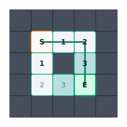
The diagram shows the wavefront on the 5×5 recap maze. The orange cell is S at distance 0. Each teal cell is labeled with its distance from S, which is the wave number on which it first got reached. The green cell is E, whose first-reach distance is 4. The line running through the grid is the parent chain. Starting from E, follow the parent pointer to (2,3), then to (1,3), then to (1,2), then back to S. Reverse that chain and you have the shortest path, length 5 cells.
public List<Position> solve() {
    Position start = maze.getStart();
    Position end = maze.getEnd();

    List<Position> queue = new ArrayList<>();
    queue.add(start);
    List<Position> visited = new ArrayList<>();
    visited.add(start);
    Map<Position, Position> parent = new HashMap<>();
    parent.put(start, null);

    while (!queue.isEmpty()) {
        Position current = queue.remove(0);

        if (current.equals(end)) {
            LinkedList<Position> path = new LinkedList<>();
            Position node = current;
            while (node != null) {
                path.addFirst(node);
                node = parent.get(node);
            }
            return path;
        }

        for (Position neighbor : maze.getNeighbors(current)) {
            boolean seen = false;
            for (Position v : visited) {
                if (v.equals(neighbor)) { seen = true; break; }
            }
            if (!seen) {
                visited.add(neighbor);
                parent.put(neighbor, current);
                queue.add(neighbor);
            }
        }
    }

    return null;
}
A few details in the code are worth tracing through. The first is that visited is marked on enqueue rather than on dequeue, so every cell flips to visited the moment it enters the queue rather than the moment it leaves. That matters because if you mark on dequeue, the same cell can be added to the queue from two different neighbors before either of those neighbors is processed, meaning multiple copies of the same cell sit on the queue simultaneously and the search re-explores it when each copy surfaces. You'd still find the right path, but the queue would balloon and you'd re-expand duplicates, whereas marking on enqueue caps the total work at one expansion per cell.
The start's parent is null (or None), which is how the path-reconstruction loop knows when to stop. You walk parent[node] until it comes back empty, and the start is the only cell for which that happens.
Finally, the path is built end-to-start and then reversed at the end. That falls out of how parent pointers work, since they only point backward toward S. You could instead build the path forward by reversing the parent graph, but reversing a finished list is cheaper and easier.
Complexity
Let V = rows × cols, which is the number of cells in the grid. BFS itself touches every reachable cell exactly once. The cost per cell depends on the containers.
- Removing from the front of a list shifts every remaining element one slot to the left. Python lists and most dynamic arrays store elements in contiguous memory indexed from 0, so popping index 0 forces every other element to shift down by one to keep the indexing consistent, which is O(n) per pop. Across a full BFS that's up to O(V) work per dequeue, or O(V²) total just for the queue.
- Checking membership in the visited list scans it end to end. That's also O(V) per check, and again O(V²) across the whole search.
- The combined total is O(V²).
Where it breaks
The small mazes are fine because V² is tiny when V is a few dozen. The huge mazes are not. On a 75×75 grid the solver takes about 305 ms, just over the 300 ms budget. On 100×100 it takes about 945 ms, nearly twice the 500 ms budget. On 150×150 it takes about 4.73 s, roughly five times the 1000 ms budget. The algorithm finds the right answer every time. It just doesn't find it fast enough.
BFS is already optimal for this problem at O(V + E), and on a 4-neighbor grid E is at most 4V (each cell borders at most four others), so the complexity simplifies to O(V) once constants drop out. The quadratic blowup has nothing to do with how many cells we visit and everything to do with the per-cell cost of touching the queue and the visited set.
Solution 2, BFS with a constant-time queue and a hash set
The two operations that hurt on the list version are the front-of-queue removal and the membership check against a growing list. Both scan the whole container. The fix is to replace each with a container that answers the same question in constant time.
A proper queue keeps pointers to both the head and the tail of its underlying storage. Dequeueing from the head advances the head pointer by one slot, enqueueing at the tail advances the tail pointer by one slot, and none of the elements in between move. Every language here reaches that shape a little differently. Some use a built-in double-ended queue, others use a ring-buffered queue class, and others use a plain array with a head index that walks forward on every dequeue. A ring buffer allocates a fixed-size array and tracks head and tail indices that wrap around modulo the capacity, so both enqueue and dequeue are O(1) without any shifting; a plain array with a head index takes a simpler approach where the front slots are just abandoned as the head advances, which grows memory over time but keeps each operation O(1). The asymptotic win is the same across all of them, since both ends now operate in constant time.
A hash set is a set backed by a hash table. To answer "is this key in the set?", the set hashes the key, jumps to the matching bucket, and checks whether the key is sitting there. It performs no scan over the stored elements. That's what amortized O(1) means for in. The cost of one lookup does not grow with the number of elements you've stored.
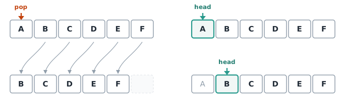
The diagram shows what each container does on a single dequeue. On the left, pulling from the front of a list forces the five elements behind it to slide over by one slot to close the gap. On the right, the dequeue just bumps a head pointer forward and leaves the slots untouched. Scaled up to a full BFS on the 150×150 maze, that difference is the gap between 4.73 seconds and 77 milliseconds.
public List<Position> solve() {
    Position start = maze.getStart();
    Position end = maze.getEnd();

    Deque<Position> queue = new ArrayDeque<>();
    queue.add(start);
    Set<Position> visited = new HashSet<>();
    visited.add(start);
    Map<Position, Position> parent = new HashMap<>();
    parent.put(start, null);

    while (!queue.isEmpty()) {
        Position current = queue.pollFirst();

        if (current.equals(end)) {
            LinkedList<Position> path = new LinkedList<>();
            Position node = current;
            while (node != null) {
                path.addFirst(node);
                node = parent.get(node);
            }
            return path;
        }

        for (Position neighbor : maze.getNeighbors(current)) {
            if (!visited.contains(neighbor)) {
                visited.add(neighbor);
                parent.put(neighbor, current);
                queue.add(neighbor);
            }
        }
    }

    return null;
}
The BFS logic is unchanged. Two container swaps and a small adjustment to how visited membership is checked.
Complexity
- BFS still touches every reachable cell once. Per-cell work is now constant because each dequeue and each visited-set lookup both run in constant time.
- Total time is O(V + E), which on a 4-neighbor grid simplifies to O(V) = O(rows × cols).
- Space is O(V) for the visited set, the parent map, and the queue combined.
Where it lands
Every huge-maze test clears its budget by at least an order of magnitude. The 75×75 runs in ~19 ms vs a 300 ms budget. The 100×100 in ~33 ms vs 500 ms. The 150×150 in ~77 ms vs 1000 ms. Because the list version's per-cell cost grows with V while the deque+set version's per-cell cost is constant, the speedup grows with the maze too, running about 16× on 75×75, 29× on 100×100, and 61× on 150×150. The intuition is that a 75×75 grid has 5,625 cells, a 100×100 has 10,000, and a 150×150 has 22,500, so successive mazes are roughly 2× and 4× larger in area; the list version's quadratic cost grows with that area while the deque version's cost stays linear, which explains why the wall-clock gap widens rather than staying proportional.
One-way passages
The shipped problem includes directional cells. > accepts entry only from its west neighbor moving east. < accepts entry only from its east neighbor moving west. Entering from any other side is blocked.
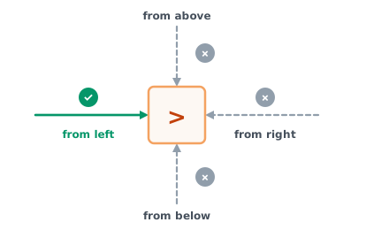
Every move into a directional cell has a direction vector (dx, dy) = (to.col - from.col, to.row - from.row). For >, the only valid direction is (1, 0). For <, the only valid direction is (-1, 0). Anything else is rejected. That check belongs on the maze itself, right next to the existing bounds and wall checks, because it needs both the source and the destination in hand. The solver code doesn't change at all. It keeps asking the maze for the legal neighbors of the current cell, and the maze is now the one place that knows about directional rules.
A tempting shortcut is to decide walkability at the cell level, either by accepting every > as open or by treating it as a wall, and then skipping the direction check entirely. Both versions are wrong. The constraint isn't a property of the cell; it's a property of the move. It can only be evaluated with both the source and the destination in hand, which is why it has to live in the neighbor-generation step rather than in whatever function classifies a single cell as walkable.
Benchmarks
All numbers are on the shipped datasets with direction-aware neighbor generation. Both variants return the same path on every dataset. Sizes below are the inner walkable area, matching how the huge-maze generators and test names are labeled.
| Maze | Size | list_bfs | deque_bfs | Path length |
|---|---|---|---|---|
| simple | 3×3 | 31 µs | 31 µs | 5 |
| small | 5×5 | 78 µs | 75 µs | 9 |
| medium | 13×13 | 298 µs | 251 µs | 26 |
| directional | 5×5 | 70 µs | 68 µs | 9 |
| directional_blocked | 3×5 | 8 µs | 8 µs | — |
| anywhere | 3×5 | 30 µs | 30 µs | 5 |
| huge_75 | 75×75 | 305 ms | 19 ms | 149 |
| huge_100 | 100×100 | 945 ms | 33 ms | 199 |
| huge_150 | 150×150 | 4.73 s | 77 ms | 299 |
Bold rows are the ones where the list variant runs over the per-test budget. On every maze under about 30×30, both variants are inside a millisecond, so if the problem only shipped small mazes, list_bfs would pass and nobody would notice the container choice. The test suite exists to expose exactly this gap.
The speedup grows with maze size because the list version's per-cell cost grows with V, which is why the gap is about 16× on 75×75 and about 61× on 150×150. The directional_blocked row is the outlier that shortcuts out almost immediately because S sits in a small enclosed region; BFS exhausts every cell reachable from S, the queue empties without ever touching E, and the solver returns null right there rather than scanning the rest of the grid.
Takeaways
Shortest-path on an unweighted graph is always BFS. No weights means no reason to reach for Dijkstra, A*, or anything fancier, and the uniform-cost moves here keep the problem squarely in that territory. The harder lesson is that picking BFS only gets you the theoretical O(V + E) if the data structures underneath actually deliver constant-time operations, and that's easy to miss when the small test cases still pass. Back the queue with something that shifts on every dequeue, or back the visited set with something that scans on every lookup, and the real cost becomes O(V²), which is quadratic enough to blow past the large-maze budgets by a factor of five.
The pattern generalizes past this problem. Any time a BFS or DFS has a bad wall-clock while its asymptotic looks right, the containers are the first suspect. The usual culprits are marking on dequeue when you should mark on enqueue, keying by reference when you should key by value, and reaching for whatever container the standard library makes easiest instead of one that actually matches the operations you're performing.