Problem Breakdown
Route Planner
Try This Problem Yourself
Practice in the AI-enabled editor with real-time feedback
You're given a Network of stations connected by edges. Each edge carries a travel time (in minutes) and a line name ("Blue", "Express", etc.). Some edges are one-way. The main planner method takes a start and end station and returns the route that minimizes total travel time, where switching lines costs an extra 5 minutes per transfer. A second planner method takes the same inputs plus a cap on how many times you can switch lines.
On the shipped test map, three routes exist from Central to Airport.
Green:  Central → Park → Airport                        4 + 6   = 10 min
Red:    Central → Harbor → Airport                      5 + 3   = 8 min
Blue:   Central → Mall → Stadium → Airport              2 + 3 + 2 = 7 min  (best)
The Blue route wins with three hops, even though by hop count you'd pick the two-hop Red route.
That transfer penalty looks like a small detail, but it's the thing the whole problem turns on. It means the cost of your next edge depends on which line you arrived on, and that single fact is what trips up every solution short of the last one.
Solution 1, BFS by hop count
BFS is the first algorithm most people reach for when they hear "shortest path". The template is short. You keep a queue of partial paths and a visited set of stations. On each step you pop the front of the queue and push every unvisited neighbor onto the back. The search stops the first time the destination comes off the queue, and that's the returned path.
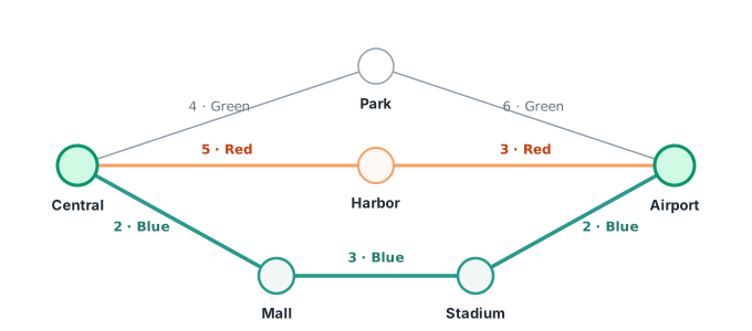
The diagram shows all three Central-to-Airport routes laid out on the shipped test map. BFS walks neighbors of Central first, then neighbors of those, and so on. Airport is reachable in two hops via the Red line and via the Green line, so BFS returns one of those (whichever lands in the queue first). The Blue route takes three hops and is the route BFS will not pick, even though it's the one with the lowest total time.
public Route findRoute(String start, String end) {
    if (!network.hasStation(start) || !network.hasStation(end)) return null;
    if (start.equals(end)) return new Route(List.of(start), 0, 0);

    record Node(String station, List<String> path, String line, int time, int transfers) {}
    Deque<Node> queue = new ArrayDeque<>();
    queue.add(new Node(start, List.of(start), null, 0, 0));
    Set<String> visited = new HashSet<>();
    visited.add(start);

    while (!queue.isEmpty()) {
        Node cur = queue.pollFirst();
        if (cur.station.equals(end)) return new Route(cur.path, cur.time, cur.transfers);
        for (Connection conn : network.getNeighbors(cur.station)) {
            if (visited.contains(conn.destination)) continue;
            visited.add(conn.destination);
            boolean isTransfer = cur.line != null && !cur.line.equals(conn.line);
            List<String> np = new ArrayList<>(cur.path);
            np.add(conn.destination);
            queue.add(new Node(
                conn.destination, np, conn.line,
                cur.time + conn.travelTime + (isTransfer ? 5 : 0),
                cur.transfers + (isTransfer ? 1 : 0)
            ));
        }
    }
    return null;
}
Every queue entry tracks the running travel time and transfer count, even though BFS ignores those weights when it picks which edge to cross next. That accumulator is why the route you return at least comes back with a correct time and transfer count, even if it isn't the fastest route.
The visited set is keyed on station alone, which is the right thing for BFS by hop count. BFS explores all stations one hop from the start before any station two hops out, so the first time a station is dequeued, its distance equals the minimum number of edges from the start. On a weighted graph that shortcut is exactly what makes BFS wrong, because fewest hops and least time are different questions.
Complexity
Let V be the number of stations and E the number of connections. Each station enters the queue at most once because of the visited set, and each edge is examined at most once per endpoint, so the traversal is O(V + E).
Where it breaks
On the shipped test map BFS returns an 8-minute Red-line route when the best real answer is 7 minutes on Blue. That's a 12% miss on a tiny graph. On the 50×50 grid the miss is larger in absolute terms, with BFS returning a 441-minute route when the true minimum is 387. The grids have per-edge travel times between 1 and 9 minutes, so a route with a few extra edges that each happen to be cheap will beat a route with fewer edges that each happen to be expensive.
The fix is to rank partial routes by their accumulated weight instead of by hop count.
Pattern: Graph Search & Pathfinding
Shortest travel time over a transit map is Dijkstra's algorithm, the weighted cousin of BFS. You expand the cheapest-so-far station first and let the priority queue do the bookkeeping.
Solution 2, Dijkstra keyed on station
The right family for non-negative weighted shortest paths is Dijkstra's algorithm. Instead of a FIFO queue, you use a min-heap keyed on cumulative time from the start. A plain queue would lock in a station at whatever path reached it first, which isn't the cheapest one once edges carry different costs. Each iteration pops the cheapest unfinished path, settles that station by locking in its time, and pushes every neighbor with its updated total.
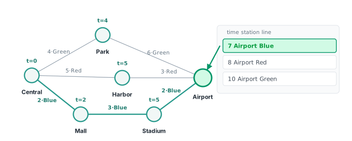
The diagram shows Dijkstra partway through Central → Airport on the shipped test map. Every intermediate station has settled at its final time, with Central at 0, Mall at 2, Park at 4, Harbor at 5, and Stadium at 5. The only thing left in the heap is three pending arrivals at Airport, and the cheapest is the Blue-line arrival at time = 7. Popping the 7 locks in Airport and the search ends with the right answer on this map.
public Route findRoute(String start, String end) {
    if (!network.hasStation(start) || !network.hasStation(end)) return null;

    record Entry(int time, long cnt, String station, String line, List<String> path, int transfers) {}
    PriorityQueue<Entry> heap = new PriorityQueue<>((a, b) ->
        a.time != b.time ? Integer.compare(a.time, b.time) : Long.compare(a.cnt, b.cnt)
    );
    long counter = 0;
    heap.add(new Entry(0, counter++, start, null, List.of(start), 0));
    Map<String, Integer> visited = new HashMap<>();

    while (!heap.isEmpty()) {
        Entry e = heap.poll();
        if (e.station.equals(end)) return new Route(e.path, e.time, e.transfers);
        Integer v = visited.get(e.station);
        if (v != null && v <= e.time) continue;
        visited.put(e.station, e.time);
        for (Connection conn : network.getNeighbors(e.station)) {
            boolean isTransfer = e.line != null && !e.line.equals(conn.line);
            List<String> np = new ArrayList<>(e.path);
            np.add(conn.destination);
            heap.add(new Entry(
                e.time + conn.travelTime + (isTransfer ? 5 : 0),
                counter++,
                conn.destination, conn.line, np,
                e.transfers + (isTransfer ? 1 : 0)
            ));
        }
    }
    return null;
}
Each heap entry carries the current line, which is how the transfer penalty gets computed on expansion. When you cross an edge, the cost is connection.travel_time plus 5 if the neighbor's line differs from the line you arrived on. A null-or-same check handles the two edge cases without a penalty, the first hop out of the start with no prior line and any later same-line hop. A monotonic counter sits in the heap tuple to break ties deterministically when two entries share a time, so the heap never has to compare the payloads.
The trouble is the visited set, which is keyed on station alone. That keying says the first time you settle a station, the cheapest arrival there is all you'll ever need. For a plain weighted graph that's true. Here it isn't, because the transfer penalty means the cost of leaving a station depends on the line you arrived on, and a station-only key throws that information away.
Where it breaks
Picture two ways to reach B. You can go Start → A → B entirely on the Red line for a total of 2 minutes, or Start → B directly on the Blue line for 3 minutes. From B there's a Blue edge to End costing 1 minute. The fastest route to End is Start → B → End, which stays on Blue the whole way for 4 minutes and zero transfers.
Station-keyed Dijkstra misses it. It settles B via the Red arrival at 2, since 2 beats 3, and records B as done. When it expands B toward End, leaving on Blue from a Red arrival costs a 5-minute transfer, so End comes out at 2 + 1 + 5 = 8. The Blue arrival at B would have continued to End with no transfer at all, but it gets discarded the moment it pops, because B is already marked visited at 2. The algorithm returns 8 when the answer is 4.
This is not a contrived edge case. On the shipped 50×50 grid, station-keyed Dijkstra returns a 389-minute route when the true minimum is 387, and it misses on the other grids too. It gets the small test map right only because that map has no place where arriving on the wrong line costs you later.
"Cheapest time to reach B" isn't enough to continue the search. You also need to know which line you got there on.
Solution 3, Dijkstra keyed on (station, line)
The fix for the plain route is to treat (station, line) as the unit of state rather than the station by itself. Two arrivals at B, one on Red and one on Blue, are two different nodes in the graph Dijkstra is searching, because the cost to continue from each one is different. Everything else about Dijkstra stays the same; only the visited map's key grows from station_id to (station_id, line_id).
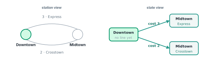
The left side of the diagram is the station view, showing two stations and two edges between them on different lines. The right side is the state view. The starting state pairs Downtown with a null line, since you haven't taken any edge yet. The other two states are Midtown reached by the Express edge and Midtown reached by the Crosstown edge. Dijkstra runs on the state view. Arrivals at the same station on different lines are genuinely separate nodes, and both get their chance to expand.
public Route findRoute(String start, String end) {
    if (!network.hasStation(start) || !network.hasStation(end)) return null;

    record Entry(int time, long cnt, String station, String line) {}
    PriorityQueue<Entry> heap = new PriorityQueue<>((a, b) ->
        a.time != b.time ? Integer.compare(a.time, b.time) : Long.compare(a.cnt, b.cnt)
    );
    long counter = 0;
    heap.add(new Entry(0, counter++, start, null));
    Map<String, Integer> best = new HashMap<>();
    Map<String, String> parent = new HashMap<>();
    Map<String, Integer> transfers = new HashMap<>();
    best.put(key(start, null), 0);
    parent.put(key(start, null), null);
    transfers.put(key(start, null), 0);

    while (!heap.isEmpty()) {
        Entry e = heap.poll();
        String sk = key(e.station, e.line);
        if (e.time > best.get(sk)) continue;
        if (e.station.equals(end)) {
            List<String> stations = new ArrayList<>();
            String cur = sk;
            while (cur != null) {
                stations.add(cur.substring(0, cur.indexOf("@@")));
                cur = parent.get(cur);
            }
            Collections.reverse(stations);
            return new Route(stations, e.time, transfers.get(sk));
        }
        for (Connection conn : network.getNeighbors(e.station)) {
            boolean isTransfer = e.line != null && !e.line.equals(conn.line);
            int newTime = e.time + conn.travelTime + (isTransfer ? 5 : 0);
            String nk = key(conn.destination, conn.line);
            if (newTime < best.getOrDefault(nk, Integer.MAX_VALUE)) {
                best.put(nk, newTime);
                parent.put(nk, sk);
                transfers.put(nk, transfers.get(sk) + (isTransfer ? 1 : 0));
                heap.add(new Entry(newTime, counter++, conn.destination, conn.line));
            }
        }
    }
    return null;
}

private static String key(String station, String line) {
    return station + "@@" + (line == null ? "" : line);
}
The visited check gates on best[state], the cheapest time recorded for that exact (station, line). Relaxing an edge offers a neighbor a new candidate time through the current state, and it updates best, parent, and the transfer count only when that time genuinely improves on what's there. That last part matters for the path you return. If you wrote the parent pointer on every push instead of only on an improvement, a worse arrival could overwrite the parent of a state before the best arrival settles, and the stations you reconstruct would no longer match the time you report.
With the line in the state, the plain route is correct everywhere. On the test map it returns 7, and on the three grids it returns the true minimums of 387, 469, and 239. The earlier counter-example now resolves the way it should, with Start → B → End coming back at 4.
Solution 4, Dijkstra keyed on (station, line, transfers)
The plain route is solved. The transfer-limited method is where (station, line) falls apart, and it's a different failure than the last one.
Imagine Start → A → B where Start → A is Red and A → B is Blue, so reaching B this way takes one transfer. The other way, Start → B directly, stays on Blue and takes zero transfers but costs more time. From B, the only edge to End is on Yellow. Now ask for the fastest route from Start to End with at most one transfer.
The valid answer is Start → B → End. It arrives at B on Blue with zero transfers used, then spends its one allowed transfer on the Blue-to-Yellow hop to End. But (station, line) keying settles B on Blue via the cheaper one-transfer arrival through A, because that arrival has a lower time. When the zero-transfer arrival at B on Blue pops later, the visited check sees the earlier, cheaper entry and discards it. The surviving state already has its one transfer spent, so the Yellow hop to End would be a second transfer and gets pruned. The search returns a null route even though a legal one exists.
Time-domination, discarding a slower arrival the moment a faster one exists, fails here because the transfer count is a constraint, not just a cost. A state that's cheaper in time but has used more transfers does not dominate a slower state that has transfers to spare, because the slower one might be the only one that can legally finish. So the transfer count has to go into the state too. The visited key becomes (station_id, line_id, transfers_used), and an arrival is only discarded when some earlier arrival at that same station, on that same line, having used the same number of transfers, was at least as fast.
public Route findRoute(String start, String end) {
    return search(start, end, Integer.MAX_VALUE);
}

public Route findRouteWithMaxTransfers(String start, String end, int maxTransfers) {
    if (maxTransfers < 0) return null;
    return search(start, end, maxTransfers);
}

private Route search(String start, String end, int maxTransfers) {
    if (!network.hasStation(start) || !network.hasStation(end)) return null;

    boolean bounded = maxTransfers != Integer.MAX_VALUE;
    record Entry(int time, long cnt, String station, String line, int used) {}
    PriorityQueue<Entry> heap = new PriorityQueue<>((a, b) ->
        a.time != b.time ? Integer.compare(a.time, b.time) : Long.compare(a.cnt, b.cnt)
    );
    long counter = 0;
    heap.add(new Entry(0, counter++, start, null, 0));
    Map<String, Integer> best = new HashMap<>();
    Map<String, String> parent = new HashMap<>();
    best.put(key(start, null, 0, bounded), 0);
    parent.put(key(start, null, 0, bounded), null);

    while (!heap.isEmpty()) {
        Entry e = heap.poll();
        String sk = key(e.station, e.line, e.used, bounded);
        if (e.time > best.get(sk)) continue;
        if (e.station.equals(end)) {
            List<String> stations = new ArrayList<>();
            String cur = sk;
            while (cur != null) {
                stations.add(cur.substring(0, cur.indexOf("@@")));
                cur = parent.get(cur);
            }
            Collections.reverse(stations);
            return new Route(stations, e.time, e.used);
        }
        for (Connection conn : network.getNeighbors(e.station)) {
            boolean isTransfer = e.line != null && !e.line.equals(conn.line);
            int newUsed = e.used + (isTransfer ? 1 : 0);
            if (newUsed > maxTransfers) continue;
            int newTime = e.time + conn.travelTime + (isTransfer ? 5 : 0);
            String nk = key(conn.destination, conn.line, newUsed, bounded);
            if (newTime < best.getOrDefault(nk, Integer.MAX_VALUE)) {
                best.put(nk, newTime);
                parent.put(nk, sk);
                heap.add(new Entry(newTime, counter++, conn.destination, conn.line, newUsed));
            }
        }
    }
    return null;
}

private static String key(String station, String line, int used, boolean bounded) {
    String base = station + "@@" + (line == null ? "" : line);
    return bounded ? base + "@@" + used : base;
}
Both planner methods now run through one helper. The plain find_route passes an infinite cap, and the helper keys on (station, line) in that case rather than (station, line, transfers), since the transfer count never gates anything when the cap can't be exceeded. The transfer-limited method passes the real cap and gets the (station, line, transfers) key. Dropping the transfer dimension when the cap is infinite is what stops a line-alternating cycle from spinning up an unbounded number of transfer states on the large grids.
The path comes back from parent pointers rather than a copied list inside every heap entry. Each time a relaxation succeeds, you record the predecessor state, and when the destination pops you walk the pointers back to the start and reverse. The path-building cost moves from every push to once at the end.
Complexity
Let V be stations, E be edges, and L be the number of distinct lines. The plain route searches (station, line) states, so it's O((V·L + E·L) log(V·L)). The transfer-limited search adds the transfer dimension, bounded by the cap T, giving O((V·L·T + E·L·T) log(V·L·T)). On the shipped maps L ≤ 6 and the caps are small, so both factors are small constants. The transfer-limited search on the 60×60 grid finishes in about 10 milliseconds.
Where it lands
Every shipped test passes, and the two adversarial maps that break the earlier solutions now resolve correctly. The plain method returns the true minimum on the test map, a second built-in map, and all three grids. The transfer-limited method returns Start → B → End on the counter-example above and handles the zero-transfer case. A negative cap comes back null, since any route uses at least zero transfers and zero already exceeds a cap below zero.
Benchmarks (Python)
The value in parentheses next to each time is the travel time the variant returned for the plain route. A ✗ marks a returned value that is wrong. The rows run from the small Central → Airport test map and the standard Downtown → Uptown map up to three random grids. Solution 4 has no column of its own, since its plain route runs the same (station, line) search and matches the last column's times.
| Dataset | BFS | Dijkstra (station-keyed) | Dijkstra (station, line) |
|---|---|---|---|
| Central → Airport (test map) | 2µs (10 ✗) | 3µs (7) | 5µs (7) |
| Downtown → Uptown (standard) | 2µs (7) | 3µs (7) | 7µs (7) |
| 50×50 corner-to-corner seed=1 | 1.1ms (441 ✗) | 5.2ms (389 ✗) | 5.3ms (387) |
| 60×60 corner-to-corner seed=2 | 1.7ms (532 ✗) | 8.3ms (476 ✗) | 7.8ms (469) |
| 50×50 interior seed=3 | 1.0ms (265 ✗) | 4.6ms (248 ✗) | 4.9ms (239) |
BFS returns the correct total on Downtown → Uptown only because that pair has a route where fewest-hops and least-time happen to coincide. Don't read it as evidence that BFS is right here.
Station-keyed Dijkstra looks fine on the two small maps and then misses on every grid, returning 389, 476, and 248 against true minimums of 387, 469, and 239. Those small maps just don't have a spot where arriving on the wrong line costs you later, so the bug stays hidden. The (station, line) keying is the cheapest keying that's actually correct for the plain route, and its extra cost over the broken version is the L factor, which is tiny here.
Takeaways
If you landed on BFS first, the move to Dijkstra is the lesson. The cue is any per-edge weight whose sum you're trying to minimize, like transit times, road distances, or pipe costs.
The bigger lesson is about state. Twice in this problem the obvious key was too coarse. Keying on station alone looked right but lost the line you arrived on, which the transfer penalty made part of the cost. Keying on (station, line) looked right for the capped variant but lost the transfer budget, which the cap made part of what's legal. Each time, the fix was to lift the missing piece into the state. When a problem's cost or its rules depend on something more than the current node, the visited key has to include that something, or it'll quietly settle a state and throw away the arrival you actually needed. Here it was the line and then the transfer count. In other problems it's (node, remaining_fuel) or (node, parity) or (row, col, direction). Figure out what the rest of the search depends on, and put it in the state.
The parent-pointer rewrite is a smaller lesson but a useful one. Inside a hot loop, every list copy inside a heap entry is work you'll do again and again. If the only reason you're carrying the path is to return it once at the end, reconstruct it once at the end instead, and write the parent only when an arrival actually improves on what you had.